Useful Notes and Equations
Before diving into the quesitons, some of the most handy notes and equations will be summarized in this section.
Configuration & C-space
Definition 2.1. The configuration of a robot is a complete specification of the position of every point of the robot. The minimum number n of real-valued coordinates needed to represent the configuration is the number of degrees of freedom (dof) of the robot. The n-dimensional space containing all possible configurations of the robot is called the configuration space (C-space). The configuration of a robot is represented by a point in its C-space.
Task Space
Is the space containing all the configurations specified by the tasks. This space is independent of the physical robot mechanism.
Workspace
Is the C-space of the end-effector of the robot. The workspace can be interpreted as the reacheable space of the end-effector.
It is also worth noticing that a dof has to be real-valued coordinates. For instance, a discrete coordinate of a coin, \({head, tail}\), cannot be a dof, because its range is not real.
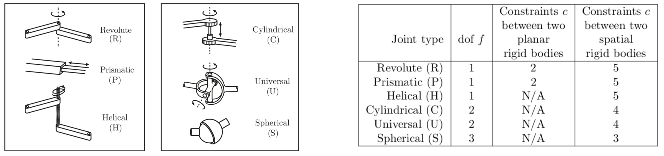
Tables
All pictures, tables, charts, unless noted otherwise, are taken from [1].
Equations
General idea about degree of freedom (DoF): \(\begin{align} \begin{split} \text{DoF} &= (\text{sum of freedoms of the points}) - (\text{No. of independent constraints})\\ &= (\text{sum of freedoms of the bodies}) - (\text{No. of independent constraints})\\ \end{split} \end{align}\)
Grübler’s Formula
\(\begin{align} \begin{split} \text{DoF} &= m(N-1)-\sum_{i=1}^{J}c_{i}\\ &= m(N-1-J)+\sum_{i=1}^{J}f_{i}\\ \text{where } m&=\text{DoF of a rigid body. For planar, m=3; for spatial, m=6}\\ N&=\text{No. of links, always add 1 to account the ground}\\ J&=\text{No. of joints}\\ c_{i}&=\text{No. of constraints provided by ith joint}\\ f_{i}&=\text{No. of DoF provided by ith joint} \end{split} \end{align}\)
N.B. that:
- Watch out for overlapping joints. If three links are connected to the same joint, then there are actually 2 joints!
- When dealing with constraints, try to model them as a special kind of joints:
- A point constraint (e.g., the end-effector must pass through a given point in space) is equivalent to a SP joint;
- A surface constraint (e.g., a block sliding on a surface) is equivalent to a RP2 joint;
- If a mechanism is consisted of purely revolute joints and have their axes of rotation meeting at a single point, then the system is actually confined to move on a surface of sphere. In this case, choose \(m = 3\).
Textbook Exercises Attempts
Exercise 2.1 Using the methods of Section 2.1 derive a formula, in terms of n, for the number of degrees of freedom of a rigid body in n-dimensional space. Indicate how many of these dof are translational and how many are rotational. Describe the topology of the C-space (e.g., for n = 2, the topology is \(\mathbb{R}^{2}\times \mathbb{S}^{1}\)).
Recall that in 3D we first choose an arbitrary point in space, which has a linear DoF of 3, then for all of the following rotational DoF, the preceding choice provides one constraint. Therefore in n=3 we have the topology \(\mathbb{R}^{3}\times \mathbb{S}^{2}\times \mathbb{S}^{1}\). Generalize this idea we have \(\mathbb{R}^{n}\times \mathbb{S}^{n-1}\times \mathbb{S}^{n-2}\times \text{...}\times \mathbb{S}^{1}\).
Exercise 2.4 Assume each of your arms has n degrees of freedom. You are driving a car, your torso is stationary relative to the car (owing to a tight seatbelt!), and both hands are firmly grasping the wheel, so that your hands do not move relative to the wheel. How many degrees of freedom does your arms-plus-steering wheel system have? Explain your answer.
The wheel is a fixed rigid body in space, therefore it adds 6 constraints to the system. Then, each of your hand has a \(DoF = n-6\). Together you have \(DoF = 2n-12\). However, if the wheel is free to rotate, then it adds 1 extra DoF to the system. In this case you have \(DoF = 2n-11\).
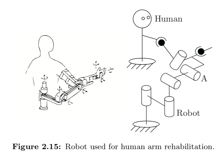
Exercise 2.5 Figure 2.15 shows a robot used for human arm rehabilitation. Determine the number of degrees of freedom of the chain formed by the human arm and the robot.
Exercise 2.6 The mobile manipulator of Figure 2.16 consists of a 6R arm and multi-fingered hand mounted on a mobile base with a single wheel. You can think of the wheeled base as the same as the rolling coin in Figure 2.11 – the wheel (and base) can spin together about an axis perpendicular to the ground, and the wheel rolls without slipping. The base always remains horizontal. (Left unstated are the means to keep the base horizontal and to spin the wheel and base about an axis perpendicular to the ground.)
- (a) Ignoring the multi-fingered hand, describe the configuration space of the mobile manipulator.
- (b) Now suppose that the robot hand rigidly grasps a refrigerator door handle and, with its wheel and base completely stationary, opens the door using only its arm. With the door open, how many degrees of freedom does the mechanism formed by the arm and open door have?
- (c) A second identical mobile manipulator comes along, and after parking its mobile base, also rigidly grasps the refrigerator door handle. How many degrees of freedom does the mechanism formed by the two arms and the open refrigerator door have?
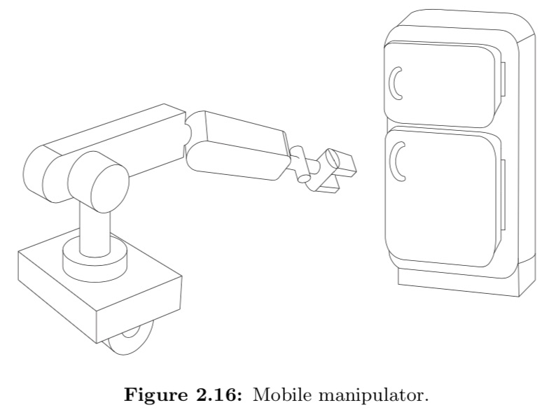
- (a) The base is kinematically equivalent to a rolling coin, then its C-space is \(\mathbb{R}^{2}\times \mathbb{T}^{2}\). The C-space of a standard 6R robot is just plainly 6 rotational DoF, i.e. \(\mathbb{S}^{1}\times ...\times \mathbb{S}^{1}=\mathbb{T}^{6}\). Altogether we have the system C-space as \(\mathbb{R}^{2}\times \mathbb{T}^{2}\times \mathbb{T}^{6}=\mathbb{R}^{2}\times \mathbb{T}^{8}\).
- (b) \(\begin{align} \begin{split} DoF &= 10(\text{total DoF})-4(\text{stationary base})\\ &-6(\text{rigid body in space})+1(\text{door been free to rotate})\\ &=1\\ \end{split} \end{align}\)
- (c) \(DoF=2\cdot(10-4-6)+1=1\)
Exercise 2.7 Three identical SRS open-chain arms are grasping a common object, as shown in Figure 2.17.
- (a) Find the number of degrees of freedom of this system.
- (b) Suppose there are now a total of n such arms grasping the object. How many degrees of freedom does this system have?
- (c) Suppose the spherical wrist joint in each of the n arms is now replaced by a universal joint. How many degrees of freedom does this system have?
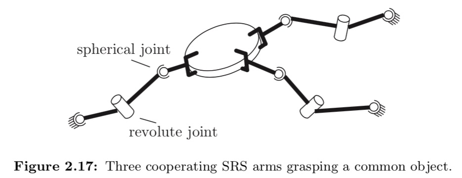
- (a) \(\begin{align} \begin{split} N &= 3\cdot(2)+1\\ J &= 3\cdot(2S+R)\\ \Sigma f_{i}&=3\cdot(2\cdot 3 +1)\\ DoF&=6\cdot (8-1+9)+21\\ &=9\\ \end{split} \end{align}\)
- (b)\(\begin{align} \begin{split} N&=2n+2\\ J&=n\cdot (2S+R)=3n\\ \Sigma f_{i}&=7n\\ DoF&=6\cdot (2n+2-1-3n)+7n\\ &=6+n\\ \end{split} \end{align}\)
- (c) S=>U, 3=>2 \(\begin{align} \begin{split} \Sigma f_{i}&=n\cdot (U+S+R)=6n\\ DoF&=6\cdot (2n+2-1-3n)+5n\\ &=6\\ \end{split} \end{align}\)
Exercise 2.8 Consider a spatial parallel mechanism consisting of a moving plate connected to a fixed plate by n identical legs. For the moving plate to have six degrees of freedom, how many degrees of freedom should each leg have, as a function of n? For example, if n = 3 then the moving plate and fixed plate are connected by three legs; how many degrees of freedom should each leg have for the moving plate to move with six degrees of freedom? Solve for arbitrary n.
\(\begin{align} \begin{split} N &= 1(moving plate) + 1(fix plate/ground)\\ J &= n\\ \text{Let x be the No. of DoF of one leg.}\\ \text{Then, }\Sigma f_{i}&=x\cdot n\\ \text{DoF}&=6\cdot (2-1-n)+x\cdot n\\ &=6\\ \end{split} \end{align}\) It seems that the DoF is a constant.
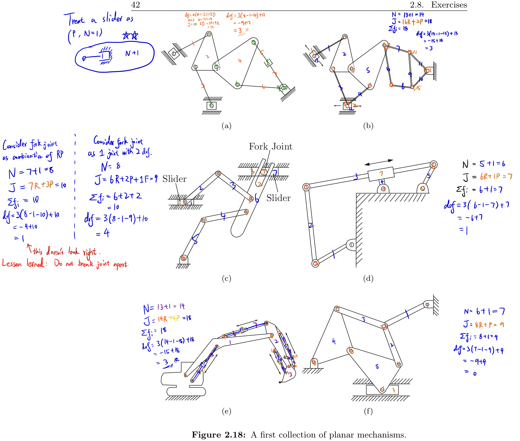
Exercise 2.9 Use the planar version of Grübler’s formula to determine the number of degrees of freedom of the mechanisms shown in Figure 2.18. Comment on whether your results agree with your intuition about the possible motions of these mechanisms.
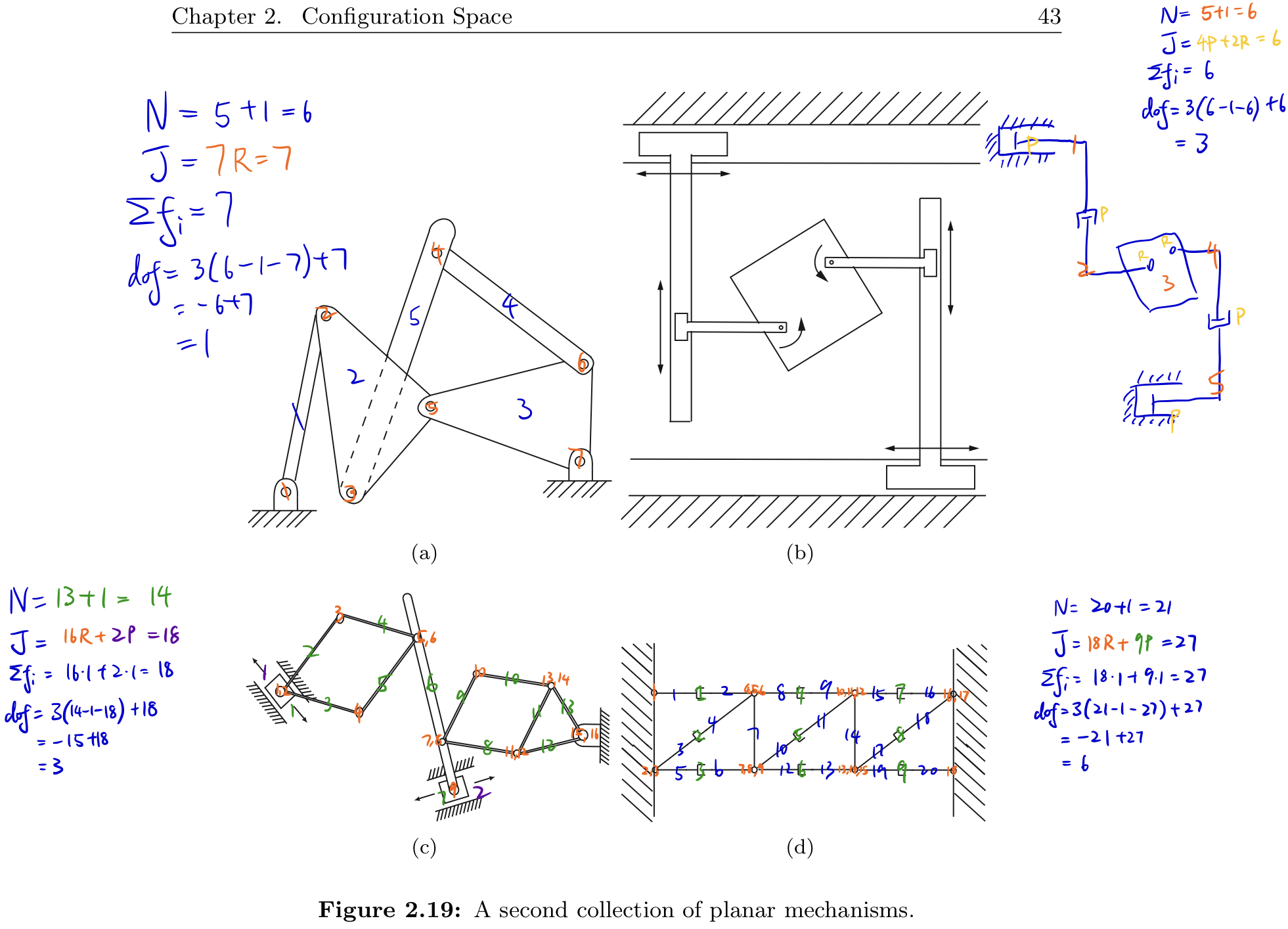
Exercise 2.10 Use the planar version of Grübler’s formula to determine the number of degrees of freedom of the mechanisms shown in Figure 2.19. Comment on whether your results agree with your intuition about the possible motions of these mechanisms.
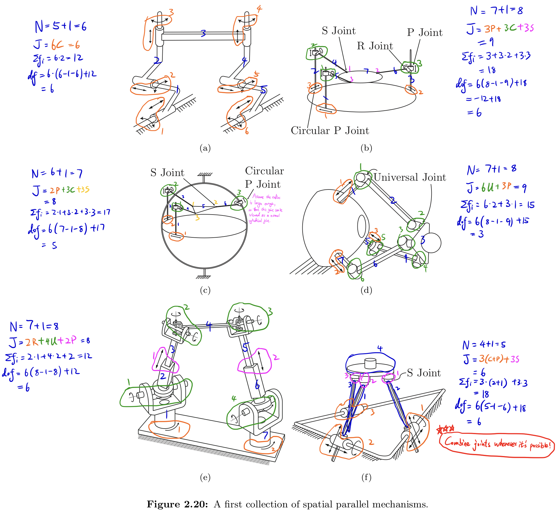
Exercise 2.11 Use the spatial version of Grübler’s formula to determine the number of degrees of freedom of the mechanisms shown in Figure 2.20. Comment on whether your results agree with your intuition about the possible motions of these mechanisms.
Exercise 2.12 Use the spatial version of Grübler’s formula to determine the number of degrees of freedom of the mechanisms shown in Figure 2.21. Comment on whether your results agree with your intuition about the possible motions of these mechanisms.
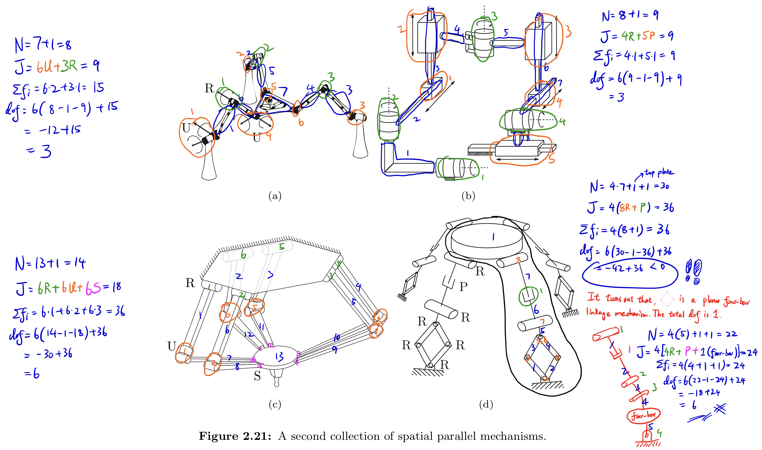
For part (d), The RRRR mechanism at the bottom is called a scissor linkage (or lazy Tongs), which is a kind of planar four-bar linkage. Such structure provides 1 DoF.
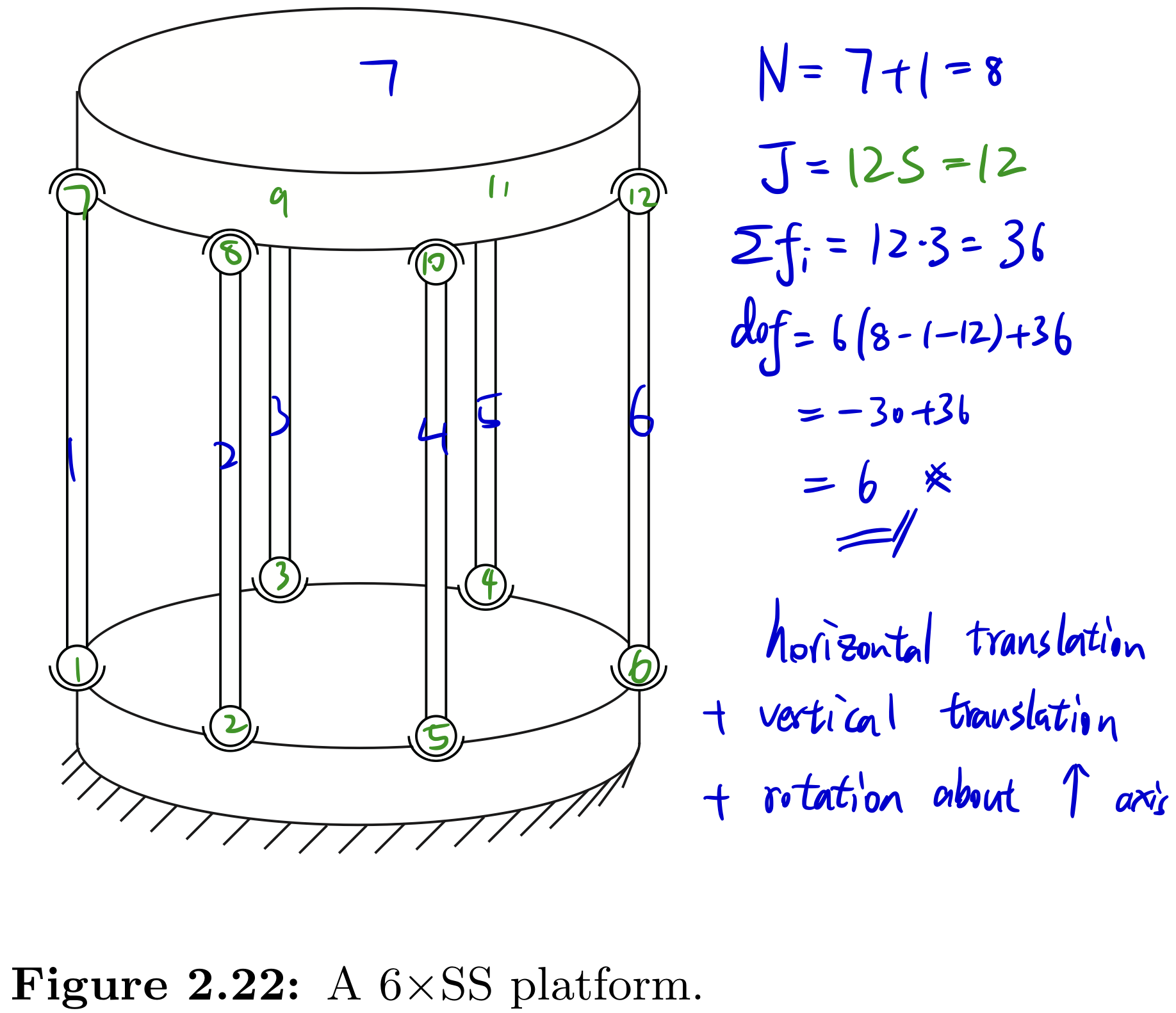
Exercise 2.13 In the parallel mechanism shown in Figure 2.22, six legs of identical length are connected to a fixed and moving platform via spherical joints. Determine the number of degrees of freedom of this mechanism using Grübler’s formula. Illustrate all possible motions of the upper platform.
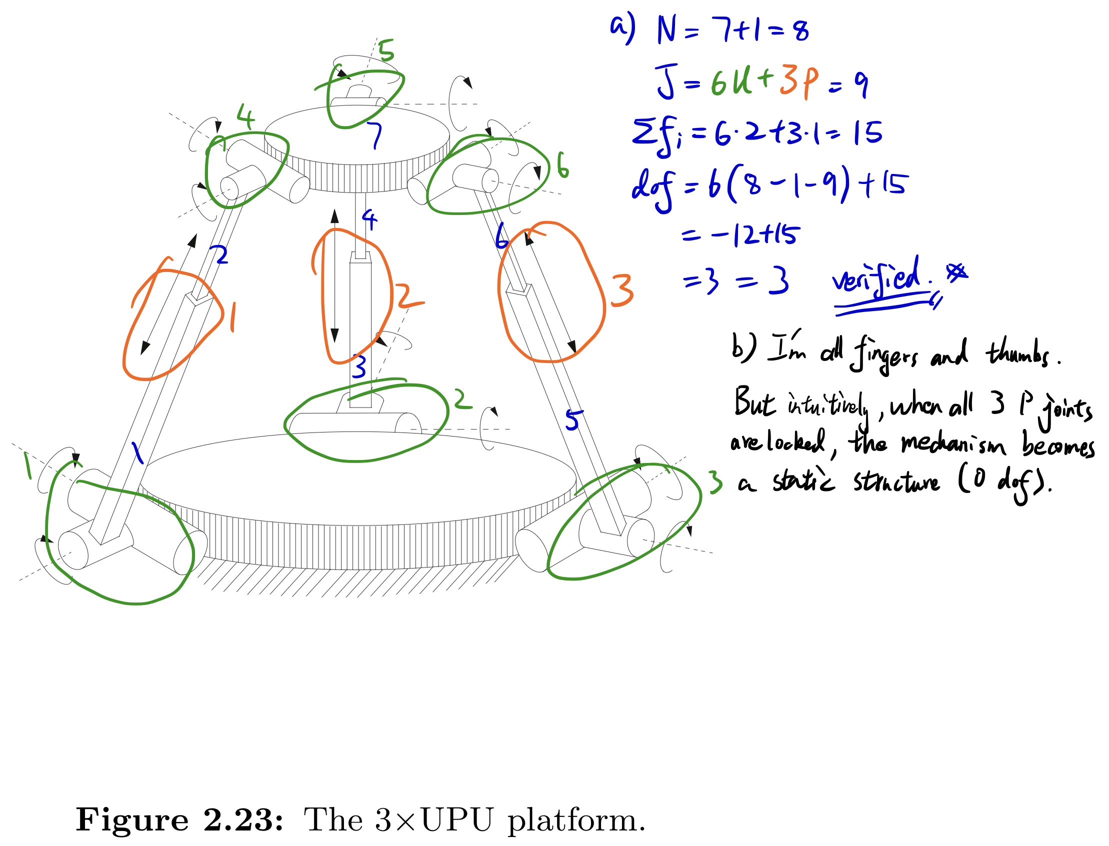
Exercise 2.14 The 3×UPU platform of Figure 2.23 consists of two platforms – the lower one stationary, the upper one mobile–connected by three UPU legs.
- (a) Using the spatial version of Grübler’s formula, verify that it has three degrees of freedom.
- (b) Construct a physical model of the 3×UPU platform to see if it indeed has three degrees of freedom. In particular, lock the three P joints in place; does the robot become a rigid structure as predicted by Grübler’s formula, or does it move?
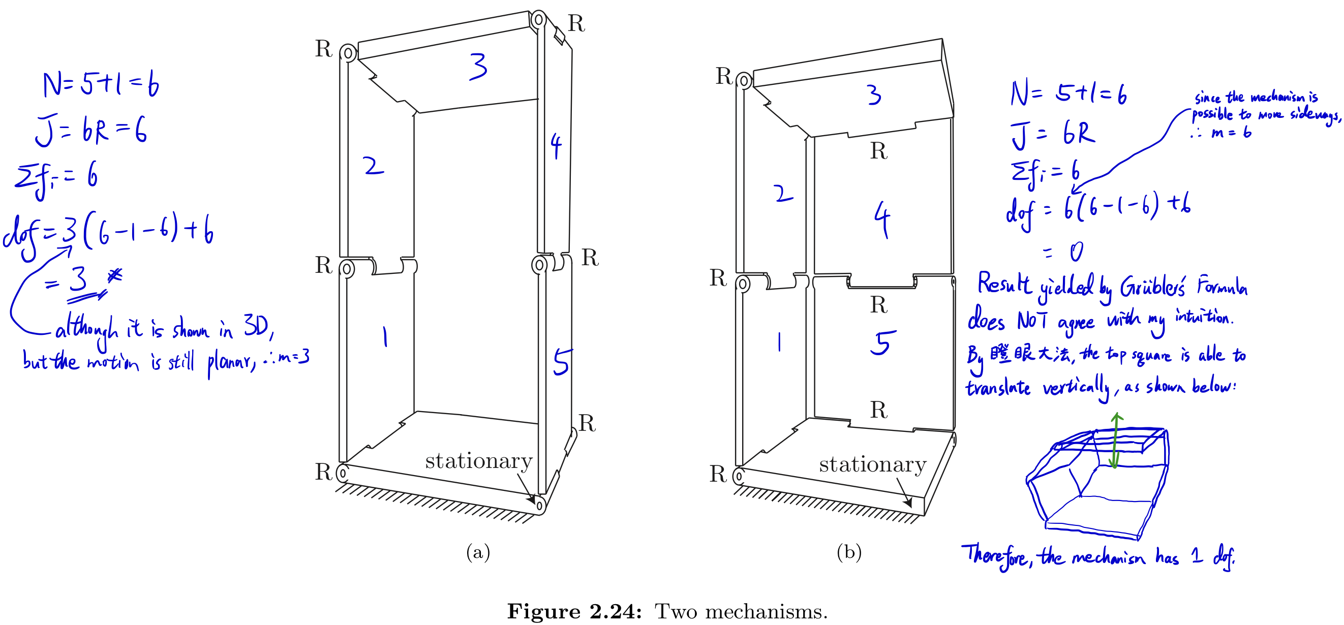
Exercise 2.15 The mechanisms of Figures 2.24(a) and 2.24(b).
- (a) The mechanism of Figure 2.24(a) consists of six identical squares arranged in a single closed loop, connected by revolute joints. The bottom square is fixed to ground. Determine the number of degrees of freedom using Grübler’s formula.
- (b) The mechanism of Figure 2.24(b) also consists of six identical squares connected by revolute joints, but arranged differently (as shown). Determine the number of degrees of freedom using Grübler’s formula. Does your result agree with your intuition about the possible motions of this mechanism?
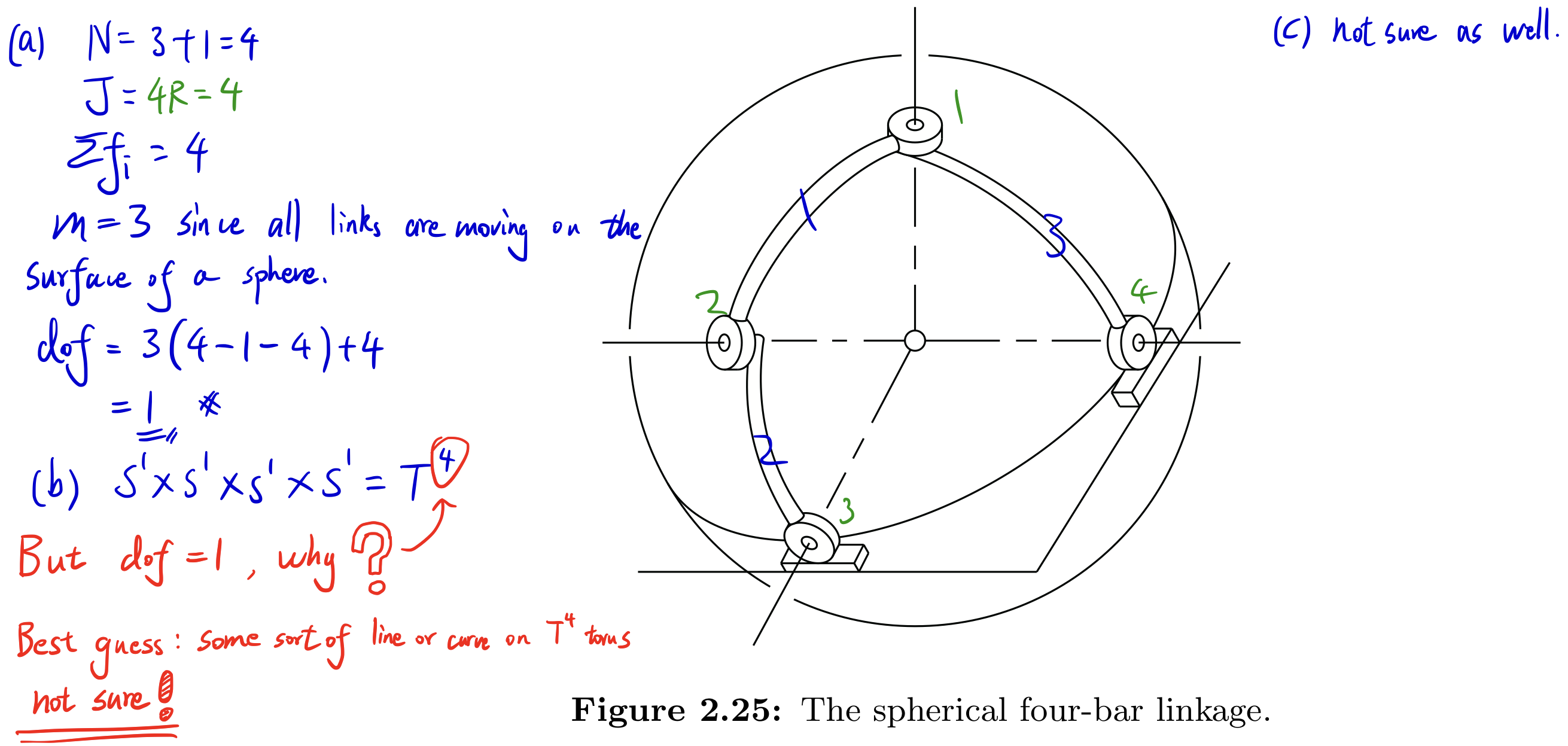
Exercise 2.16 Figure 2.25 shows a spherical four-bar linkage, in which four links (one of the links is the ground link) are connected by four revolute joints to form a single-loop closed chain. The four revolute joints are arranged so that they lie on a sphere such that their joint axes intersect at a common point.
- (a) Use Grübler’s formula to find the number of degrees of freedom. Justify your choice of formula.
- (b) Describe the configuration space.
- (c) Assuming that a reference frame is attached to the center link, describe its workspace.
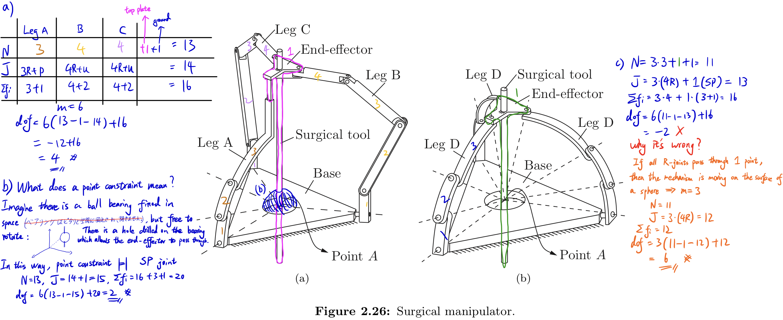
Exercise 2.17 Figure 2.26 shows a parallel robot used for surgical applications. As shown in Figure 2.26(a), leg A is an RRRP chain, while legs B and C are RRRUR chains. A surgical tool is rigidly attached to the end-effector.
- (a) Use Grübler’s formula to find the number of degrees of freedom of the mechanism in Figure 2.26(a).
- (b) Now suppose that the surgical tool must always pass through point A in Figure 2.26(a). How many degrees of freedom does the manipulator have?
- (c) Legs A, B, and C are now replaced by three identical RRRR legs as shown in Figure 2.26(b). Furthermore, the axes of all R joints pass through point A. Use Gru ̈bler’s formula to derive the number of degrees of freedom of this mechanism.
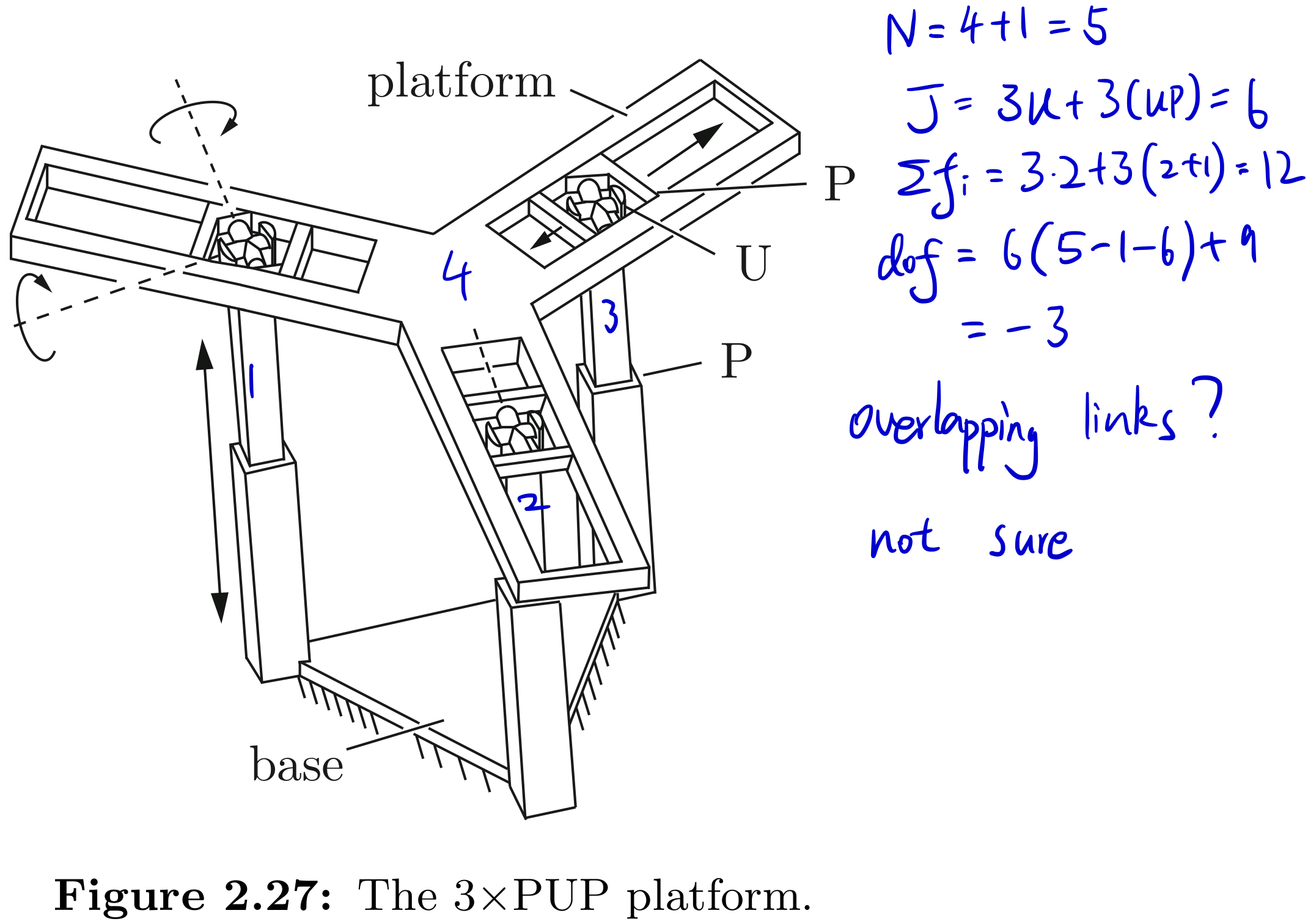
Exercise 2.18 Figure 2.27 shows a 3×PUP platform, in which three identical PUP legs connect a fixed base to a moving platform. The P joints on both the fixed base and moving platform are arranged symmetrically. Use Grbler’s formula to find the number of degrees of freedom. Does your answer agree with your intuition about this mechanism? If not, try to explain any discrepancies without resorting to a detailed kinematic analysis.
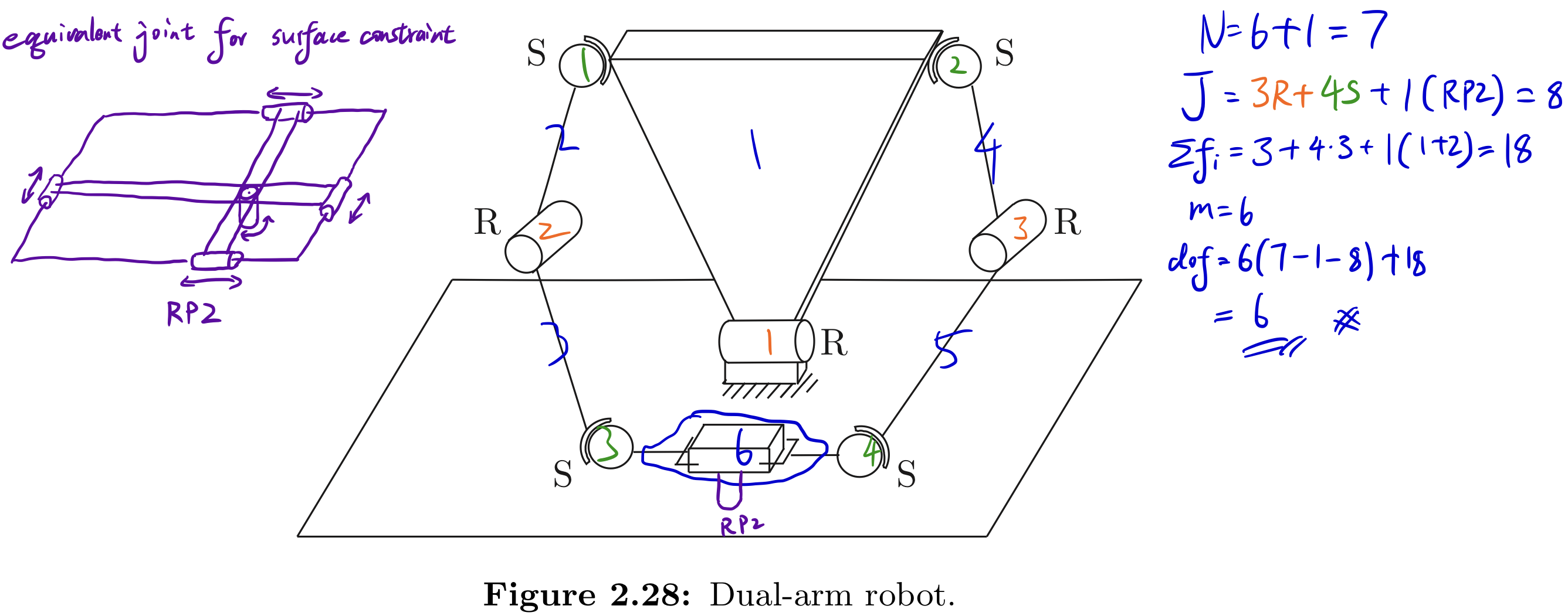
Exercise 2.19 The dual-arm robot of Figure 2.28 is rigidly grasping a box. The box can only slide on the table; the bottom face of the box must always be in contact with the table. How many degrees of freedom does this system have?
Exercise 2.20 The dragonfly robot of Figure 2.29 has a body, four legs, and four wings as shown. Each leg is connected to each adjacent leg by a USP linkage. Use Grübler’s formula to answer the following questions.
- (a) Suppose the body is fixed and only the legs and wings can move. How many degrees of freedom does the robot have?
- (b) Now suppose the robot is flying in the air. How many degrees of freedom does the robot have?
- (c) Now suppose the robot is standing with all four feet in contact with the ground. Assume that the ground is uneven and that each foot–ground contact can be modeled as a point contact with no slip. How many degrees of freedom does the robot have? Explain your answer.
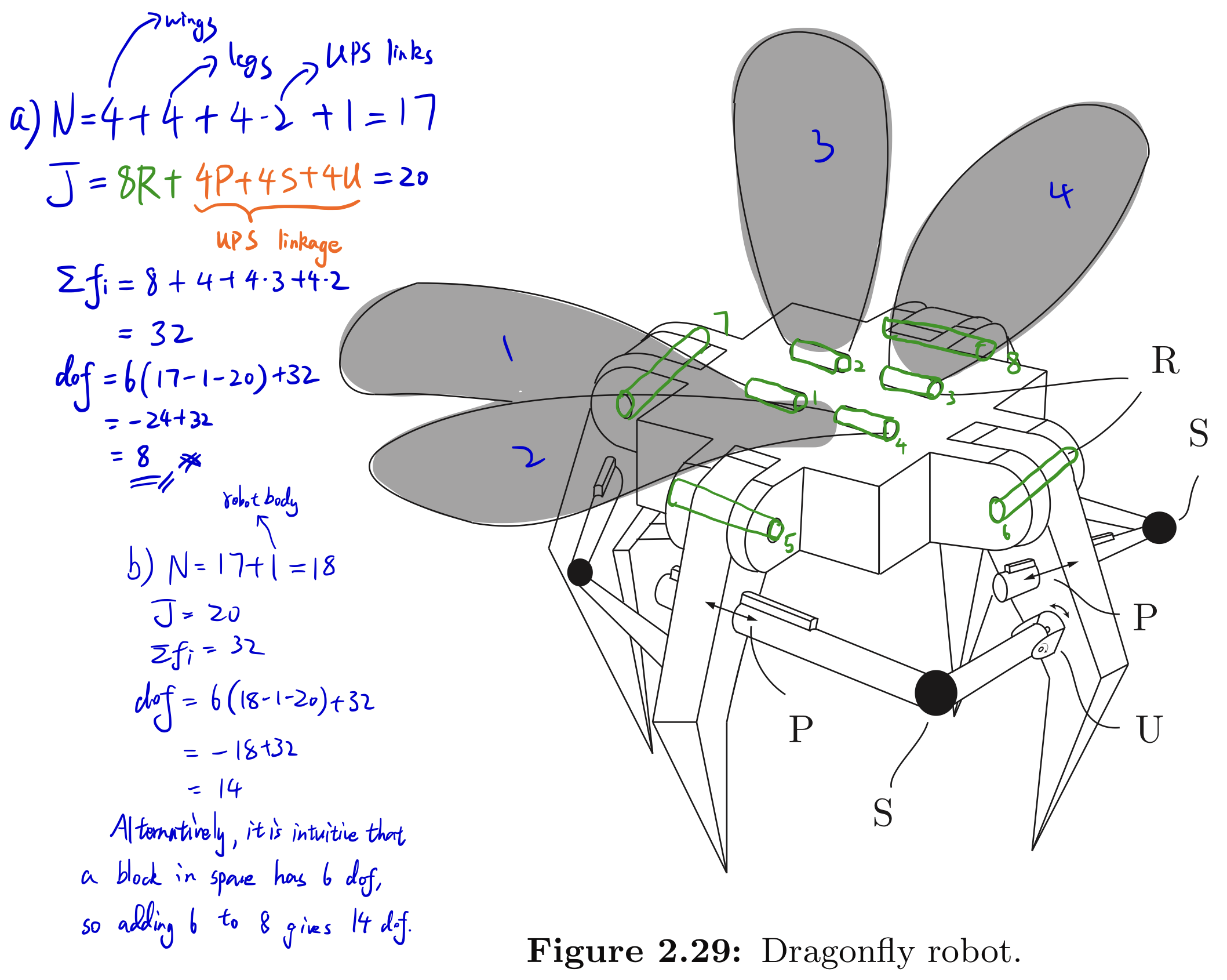
- (c) The legs on the ground can be viewed as a point constraint that does not allow translation, therefore it can be modeled as merely a S joint. In doing so, by Grübler’s formula we have:
It should be pointed out that the wings of the Dragonfly are free to move. This means that the wings have 4 DoF, while the entire system only has 2. It might imply that the rest of the system has negative DoF. I am not sure whether this is showing that the existence of dependent joints (in this case the Grübler’s formula will give negative DoF), or it is showing that there are extra constraints applied to the system.
Exercise 2.23 Consider the slider–crank mechanism of Figure 2.4(b). A rotational motion at the revolute joint fixed to ground (the “crank”) causes a translational motion at the prismatic joint (the “slider”). Suppose that the two links connected to the crank and slider are of equal length. Determine the configuration space of this mechanism, and draw its projected version on the space defined by the crank and slider joint variables.
.jpg)
Let \((x_{1}, y_{1})\), \((x_{2}, y_{2})\), \((x_{3}, y_{3})\) be the centre of the three links respectively. Let x be
\[x = \begin{bmatrix} x_{1} \\ y_{1} \\ x_{2} \\ y_{2} \\ x_{3} \\ y_{3} \\ \theta_{1} \\ \theta_{2} \end{bmatrix}\]Then, let the constraint equations \(g_{i}(x)\) be
\[g_{i}(x) = \begin{bmatrix} x_{1}-\frac{L}{2}\cos{\theta_{1}} \\ y_{1}-\frac{L}{2}\sin{\theta_{1}} \\ x_{2}-L \cos{\theta_1} - \frac{L}{2}\cos{\theta_{2}} \\ y_{2}-L \sin{\theta_1} + \frac{L}{2}\sin{\theta_{2}} \\ x_{3} - L \cos{\theta_{1}} - L \cos{\theta_{2}} \\ y_{3} - L \sin{\theta_{1}} + L \sin{\theta_{2}} \\ y_{1} \end{bmatrix} = \vec{0}\]The C-space is then defined as
\[\text{C-space} = \{x | g_{i}(x)\}\]Not sure of what is the question asking for the projection.
Exercise 2.26 The tip coordinates for the two-link planar 2R robot of Figure 2.33 are given by \(\begin{align} \begin{split} x&=2\cos{\theta_{1}} +\cos(\theta_{1}+\theta_{2})\\ y &= 2 \sin{\theta_{1}} + \sin{\theta_{1} + \theta_{2}}\\ \end{split} \end{align}\)
- (a) What is the robot’s configuration space?
- (b) What is the robot’s workspace (i.e., the set of all points reachable by the tip)?
- (c) Suppose infinitely long vertical barriers are placed at x = 1 and x = −1. What is the free C-space of the robot (i.e., the portion of the C-space that does not result in any collisions with the vertical barriers)?
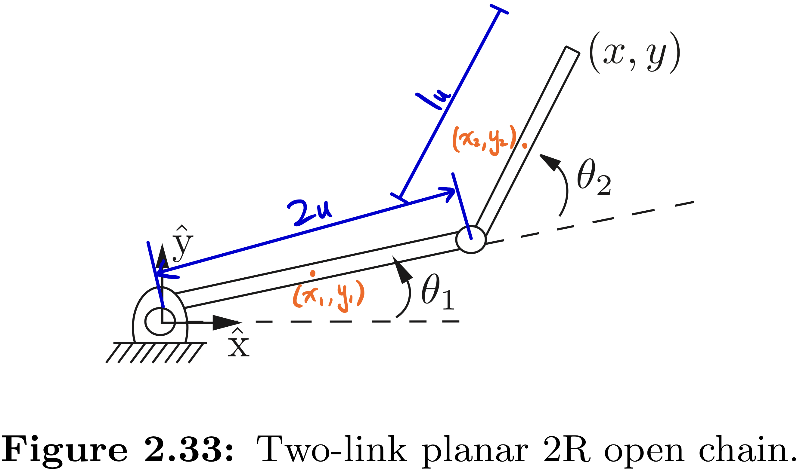
- (a) Let \((x_{1},y_{1})\) and \((x_{2},y_{2})\) be the centre of the two links respectively. Define vector \(q\) as
The constraint equations \(g_{i}(x)\) can be defined as
\[g_{i}(x) = \begin{bmatrix} x_{1} - \frac{2}{2} \cos{\theta_{1}} \\ y_{1} - \frac{2}{2} \sin{\theta_{2}} \\ x_{2} - 2 \cos{\theta_{1}} - \frac{1}{2} \cos{\theta_{1}+\theta_{2}} \\ y_{2} - 2 \sin{\theta_{1}} - \frac{1}{2} \sin{\theta_{1}+\theta_{2}} \\ \end{bmatrix} = \vec{0}\]The C-space can therefore be defined as
\[\text{C-space} = \{q | g_{i}(x)\}\]-
(b) The workspace can be defined as \(\text{Workspace} = \{ (x,y) | x=2c_{1}+c_{12}\text{, } y=2s_{1}+s_{12}, \theta_{i} \in (0,2\pi) \}\)
-
(c) The reacheable space is shown below in the sketch:
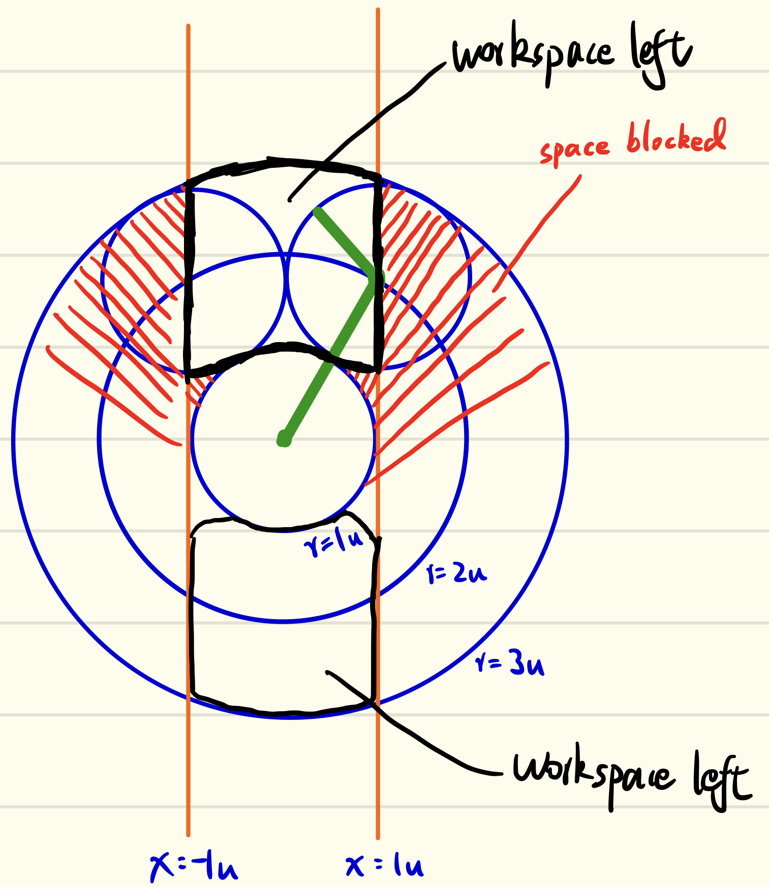
With some math, the ratio of free C-space on original C-space can be calculated. The calculation is skipped here.
Exercise 2.28 Task space.
- (a) Describe the task space for a robot arm writing on a blackboard.
- (b) Describe the task space for a robot arm twirling a baton.
- (a) A chalk in contact with the blackboard is an object on surface, therefore immediately we have \(\mathbb{R}^{2}\). Then, the orientation of the chalk will affect the sharpness of the drawing, therefore we now have \(\mathbb{R}^{2}\times \mathbb{S}^{2}\). Trivially, rotating the chalk about its central axis will not affect the drawing, thus the final task space is just \(\mathbb{R}^{2}\times \mathbb{S}^{2}\).
- (b) Not sure what does ‘twirling a baton’ refer to.
Exercise 2.29 Give a mathematical description of the topologies of the C-spaces of the following systems. Use cross products, as appropriate, of spaces such as a closed interval \([a,b]\) of a line and \(\mathbb{R}^{k}\), \(\mathbb{S}^{m}\), and \(\mathbb{T}^{n}\), where k, m, and n are chosen appropriately.
- (a) The chassis of a car-like mobile robot rolling on an infinite plane.
- (b) The car-like mobile robot (chassis only) driving around on a spherical asteroid.
- (c) The car-like mobile robot (chassis only) on an infinite plane with an RRPR robot arm mounted on it. The prismatic joint has joint limits, but the revolute joints do not.
- (d) A free-flying spacecraft with a 6R arm mounted on it and no joint limits.
- (a) \(\mathbb{R}^{2}\times \mathbb{S}^{1}\)
- (b) \(\mathbb{S}^{2}\times \mathbb{S}^{1}\)
- (c) It will be (chassis on plane) times (the RRR joints) times (the limited P joint): \(\mathbb{R}^{2}\times \mathbb{S}^{1} \times \mathbb{S}^{1}\times \mathbb{S}^{1}\times \mathbb{S}^{1} \times [a,b]= \mathbb{R}^{2}\times \mathbb{T}^{4}\times [a,b]\)
- (d) It will be (rigid body in space) times (6R arm): \(\mathbb{R}^{3}\times \mathbb{S}^{2} \times \mathbb{S}^{1} \times \mathbb{T}^{6} = \mathbb{R}^{3}\times \mathbb{S}^{2} \times \mathbb{T}^{7}\)
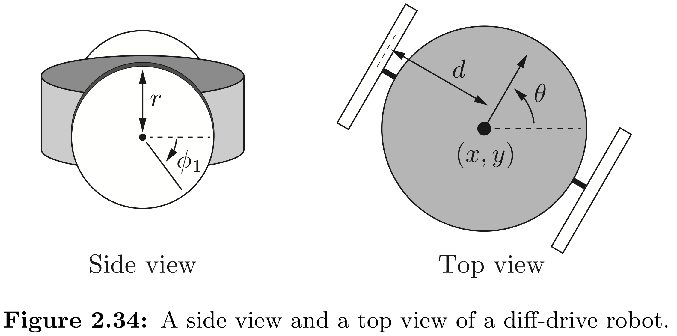
Exercise 2.31 A differential-drive mobile robot has two wheels that do not steer but whose speeds can be controlled independently. The robot goes forward and backward by spinning the wheels in the same direction at the same speed, and it turns by spinning the wheels at different speeds. The configuration of the robot is given by five variables: the \((x, y)\) location of the point halfway between the wheels, the heading direction \(\theta\) of the robot’s chassis relative to the x-axis of the world frame, and the rotation angles \(\phi_{1}\) and \(\phi_{2}\) of the two wheels about the axis through the centers of the wheels (Figure 2.34). Assume that the radius of each wheel is r and the distance between the wheels is 2d.
- (a) Let q = (x, y, \(\theta\), \(\phi_{1}\), \(\phi_{2}\)) be the configuration of the robot. If the two control inputs are the angular velocities of the wheels \(\omega_{1} = \dot{\phi_{1}}\) and \(\omega_{2} = \dot{\phi_{2}}\), write down the vector differential equation \(\dot{q} = g_{1}(q)\omega_{1} + g_{2}(q)\omega_{2}\). The vector fields \(g_{1}(q)\) and \(g_{2}(q)\) are called control vector fields (see Section 13.3) and express how the system moves when the respective unit control signal is applied.
- (b) Write the corresponding Pfaffian constraints \(A(q)\dot{q} = \theta\) for this system. How many Pfaffian constraints are there?
- (c) Are the constraints holonomic or nonholonomic? Or how many are holo- nomic and how many nonholonomic?
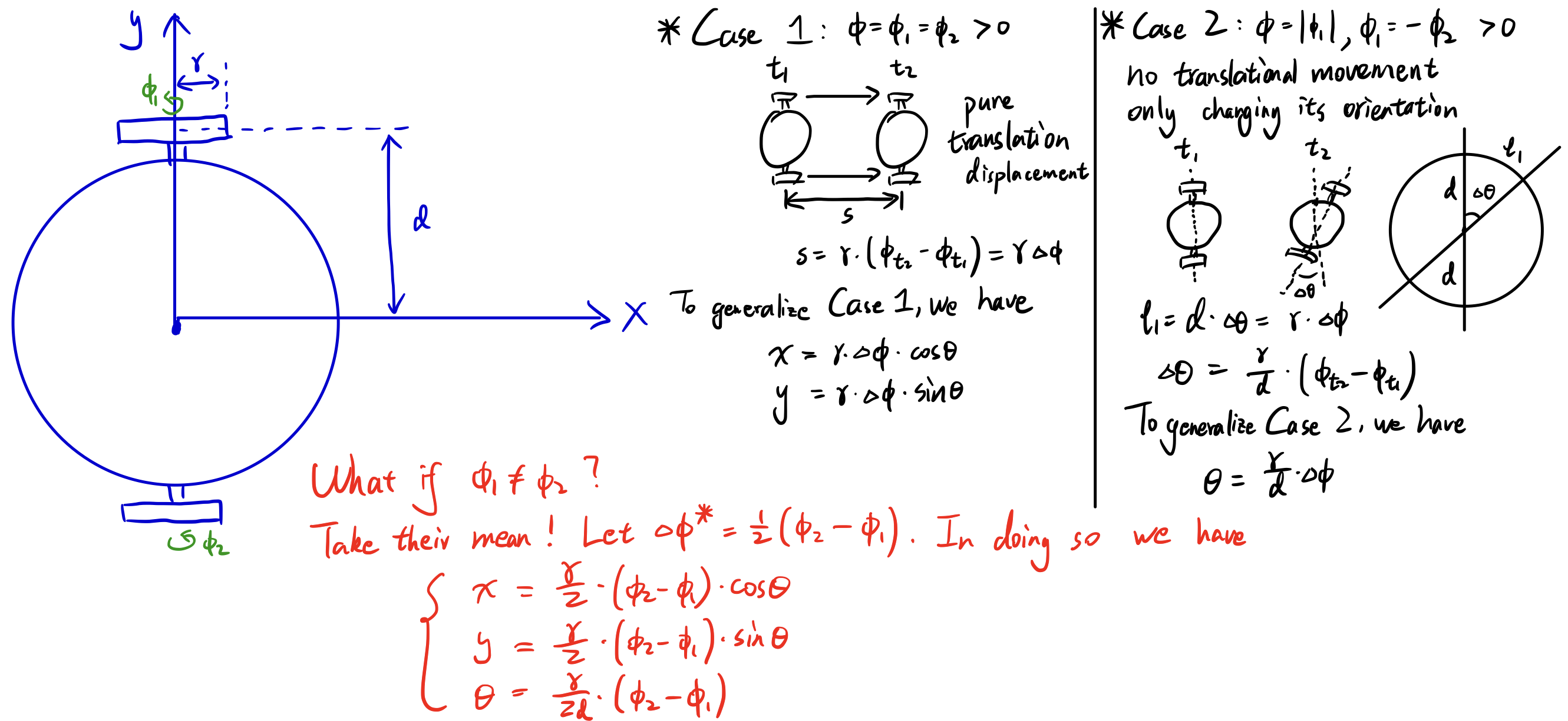
- (a) The derivation of vector q in terms of \(\phi_{1}\) and \(\phi_{2}\) is shown below in the sketch:
For a more detailed derivation, check this note.
Based on that, we get
\[\begin{align} \begin{split} \dot{q} &= \begin{bmatrix} \dot{x}\\ \dot{y}\\ \dot{\theta}\\ \dot{\phi_{1}}\\ \dot{\phi_{2}} \end{bmatrix} = \begin{bmatrix} \frac{r}{2}(\omega_{1}+\omega_{2})\cos{\theta}\\ \frac{r}{2}(\omega_{1}+\omega_{2})\sin{\theta}\\ \frac{r}{2d}(\omega_{2}-\omega_{1})\\ \omega_{1}\\ \omega_{2} \end{bmatrix}\\ \end{split} \end{align}\]Rearrange the above equation as
\[\dot{q} = \begin{bmatrix} \frac{r}{2}\cos{\theta} & \frac{r}{2}\cos{\theta}\\ \frac{r}{2}\sin{\theta} & \frac{r}{2}\sin{\theta}\\ -\frac{r}{2d} & \frac{r}{2d}\\ 1 & 0\\ 0 & 1\\ \end{bmatrix} \cdot \begin{bmatrix} \omega_{1}\\ \omega_{2}\\ \end{bmatrix}\]- (b) The Pfaffian form can be expressed as
There are 3 Pfaffian constraits.
- (c) Not sure, it seems to me that all 3 Pfaffian constraints are integratable, since they are derived by differentiation. If it is really so, then all constraints are holonomic.
This is the end of Kapitel II Exercise Attempts.
\[\begin{align*} \begin{split} \text{Valete discipulae et discipuli} \end{split} \end{align*}\]References
[1] Modern Robotics Textbook.